3.2 Creating Data Types
In the last section we explained how to use our own data types in Python. In this section we explain how to implement them.
In Python, we implement a data type using a class. Implementing a data type as a Python class is not very different from implementing a function module as a set of functions. The primary differences are that we associate values (in the form of instance variables) with methods and that each method call is associated with the object used to invoke it.
Basic Elements of a Data Type
To illustrate the process of implementing a data type as a Python class, we now consider an implementation of the Charge data type of Section 3.1.
API.
We repeat below the Charge API. We have already looked at APIs as specifications of how to use data types in client code; now look at them as specifications of how to implement data types.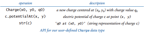
Class.
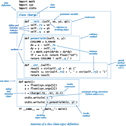
In Python, we implement a data type as a class. We define theCharge class in a file named charge.py. To define a class, we use the keyword class, followed by the class name, followed by a colon, and then a list of method definitions. Our class defines a constructor, instance variables, and methods, which we will address in detail next.
Constructor.
A constructor creates an object of the specified type and returns a reference to that object. For our example, the client code
returns a new Charge object, suitably initialized. Python provides a flexible and general mechanism for object creation, but we adopt a simple subset that well serves our style of programming. Specifically, in this booksite, each data type defines a special method __init__() whose purpose is to define and initialize the instance variables, as described below. The double underscores before and after the name are your clue that it is "special" — we will be encountering other special methods soon.
When a client calls a constructor, Python's default construction process creates a new object of the specified type, calls the __init__() method to define and initialize the instance variables, and returns a reference to the new object. In this booksite, we refer to __init__() as the constructor for the data type, even though it is technically only the pertinent part of the object-creation process.
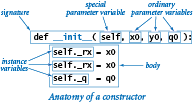
The code at right is the __init__() implementation for Charge. It is a method, so its first line is a signature consisting of the keyword def, its name (__init__), a list of parameter variables, and a colon. By convention, the first parameter variable is named self. As part of Python's default object creation process, the value of the self parameter variable when __init()__ is invoked is a reference to the newly created object. The ordinary parameter variables from the client follow the special parameter variable self. The remaining lines make up the body of the constructor. Our convention throughout this book is for __init()__ to consist of code that initializes the newly created object by defining and initializing the instance variables.
Instance variables.
A data type is a set of values and a set of operations defined on those values. In Python, instance variables implement the values. An instance variable belongs to a particular instance of a class — that is, to a particular object. In this booksite, our convention is to define and initialize each instance variable of the newly created object in the constructor and only in the constructor. The standard convention in Python programs is that instance variable names begin with an underscore. In our implementations, you can inspect the constructor to see the entire set of instance variables. For example, the__init__() implementation on the previous page tells us that Charge has three instance variables _rx, _ry, and _q. When an object is created, the value of the self parameter variable of the __init__() method is a reference to that object. Just as we can call a method for a charge c with the syntax c.potentialAt(), so we can refer to an instance variable for a charge self with the syntax self._rx. Therefore the three lines within the __init__() constructor for Charge define and initialize _rx, _ry, and _q for the new object.
Details of object creation.
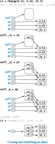
The memory diagrams at the right detail the precise sequence of events when a client creates a newCharge object with the code
- Python creates the object and calls the
__init__()constructor, initializing the constructor'sselfparameter variable to reference the newly created object, itsx0parameter variable to reference 0.51, itsy0parameter variable to reference 0.63, and itsq0parameter variable to reference 21.3. - The constructor defines and initializes the
_rx,_ry, and_qinstance variables within the newly created object referenced by self. - After the constructor finishes, Python automatically returns to the client the self reference to the newly created object.
- The client assigns that reference to
c1.
The parameter variables x0, y0, and q0 go out of scope when __init__() is finished, but the objects they reference are still accessible via the new object's instance variables.
Methods.
To define methods, we compose code that is precisely like the code that we learned in Chapter 2 to define functions, with the (significant) exception that methods can also access instance variables. For example, the code of thepotentialAt() method for our Charge data type is shown here:
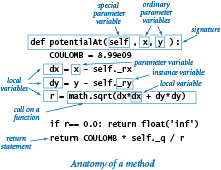
The first line is the method's signature: the keyword def, the name of the method, parameter variables names in parentheses, and a colon. The first parameter variable of every method is named self. When a client calls a method, Python automatically sets that self parameter variable to reference the object to be manipulated — the object that was used to invoke the method. For example, when a client calls our method with c.potentialAt(x, y), the value of the self parameter variable of the potentialAt() method is set to c. The ordinary parameter variables from the client (x and y, in this case) follow the special parameter variable self. The remaining lines make up the body of the potentialAt() method.
Variables within methods.
To understand method implementations, it is very important to know that a method typically uses three kinds of variables:- The
selfobject's instance variables - The method's parameter variables
- Local variables
The differences between the three kinds of variables are a key to object-oriented programming and are summarized in this table:
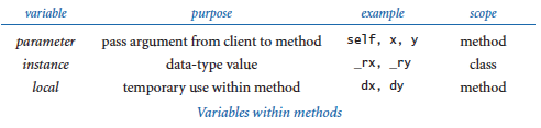
In our example, potentialAt() uses the _rx, _ry, and _q instance variables of the object referenced by self, the parameter variables x and y, and the local variables COULOMB, dx, dy, and r to compute and return a value.
Methods are functions.
A method is a special kind of function that is defined in a class and associated with an object. The key difference between functions and methods is that a method is associated with a specified object, with direct access to its instance variables.Built-in functions.
The third operation in theCharge API is a built-in function str(c). Python's convention is to automatically translate this function call to a standard method call c.__str()__. Thus, to support this operation, we implement the special method __str__(), which uses the instance variables associated with the invoking object to string together the desired result.
Privacy.
A client should access a data type only through the methods in its API. Sometimes it is convenient to define helper methods in the implementation that are not intended to be called directly by the client. The special method__str__() is a prototypical example. As we saw in Section 2.2 with private functions, the standard Python convention is to name such methods with a leading underscore. The leading underscore is a strong signal to the client not to call that private method directly. Similarly, naming instance variables with a leading underscore signals to the client not to access such private instance variables directly. Even though Python has no language support for enforcing these conventions, most Python programmers treat them as sacrosanct.
The implementation of the Charge data type in charge.py illustrates all of the features that we have described, and also defines a test client. This diagram relates the code in charge.py to its features:
For the rest of this section, we apply these basic steps to create a number of interesting data types and clients.
Stopwatch
The program stopwatch.py defines a Stopwatch class which implements this API:
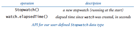
A Stopwatch object is a stripped-down version of an old-fashioned stopwatch. When you create one, it starts running, and you can ask it how long it has been running by invoking the method elapsedTime().
Histogram
The program histogram.py defines a Histogram class for graphically representing the distribution of data using bars of different heights in a chart known as a histogram. This is its API:
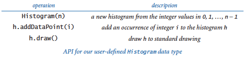
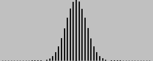
A Histogram object maintains an array of the frequency of occurrence of integer values in a given interval. Its draw() method scales the drawing so that the tallest bar fits snugly in the canvas, and then calls stdstats.plotBars() to display a histogram of the values.
% python histogram.py 50 .5 100000
Turtle Graphics
Imagine a turtle that lives in the unit square and draws lines as it moves. It can move a specified distance in a straight line, or it can rotate left (counterclockwise) a specified number of degrees. According to this API:
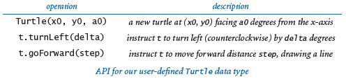
when we create a turtle, we place it at a specified point, facing a specified direction. Then, we create drawings by giving the turtle a sequence of goForward() and turnLeft() commands.
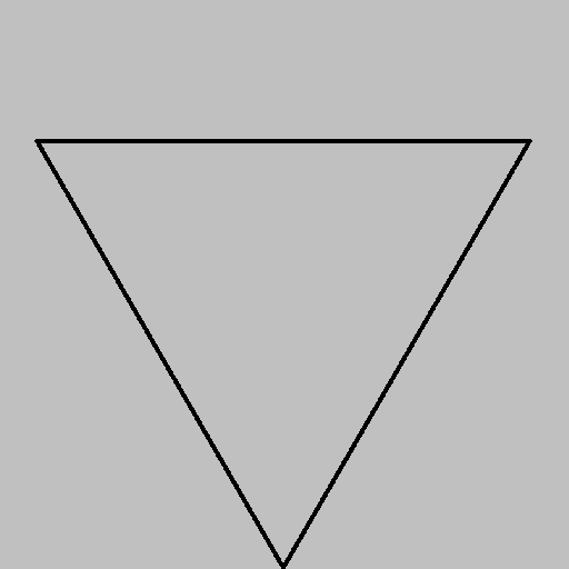
For example, to draw a triangle we create a turtle at (0, 0.5) facing at an angle of 60 degrees counterclockwise from the x-axis, then direct it to take a step forward, then rotate 120 degrees counterclockwise, then take another step forward, then rotate another 120 degrees counterclockwise, and then take a third step forward to complete the triangle.
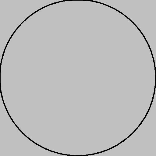
The Turtle class defined in turtle.py is an implementation of this API that uses stddraw. It maintains three instance variables: the coordinates of the turtle's position and the current direction it is facing, measured in degrees counterclockwise from the x-axis (polar angle). Implementing the two methods requires updating the values of these variables, so Turtle objects are mutable. The necessary updates are straightforward: turnLeft(delta) adds delta to the current angle, and goForward(step) adds the step size times the cosine of its argument to the current x-coordinate and the step size times the sine of its argument to the current y-coordinate. The test client in Turtle takes an integer n as a command-line argument and draws a regular polygon with n sides.
% python turtle.py 3% python turtle.py 7% python turtle.py 1000

Koch curves.
A Koch curve of order 0 is a straight line. To form a Koch curve of order n, draw a Koch curve of order n - 1, turn left 60 degrees, draw a second Koch curve of order n - 1, turn right 120 degrees (left -120 degrees), draw a third Koch curve of order n - 1, turn left 60 degrees, and draw a fourth Koch curve of order n - 1. These recursive instructions lead immediately to the turtle client code shown in koch.py. With appropriate modifications, recursive schemes like this have proved useful in modeling self-similar patterns found in nature, such as snowflakes.
% python koch.py 0% python koch.py 1% python koch.py 2% python koch.py 3% python koch.py 4


Spira mirabilis.
Imagine that the turtle's step size decays by a tiny constant factor (close to 1) each time it takes a step. What happens to our drawings? Remarkably, modifying the polygon-drawing test client in turtle.py to answer this question leads to an image known as a logarithmic spiral, a curve that is found in many contexts in nature. The program spiral.py is an implementation of this curve. The script takes three command-line arguments, which control the shape and nature of the spiral.
% python spiral.py 3 1 1.0% python spiral.py 3 10 1.2% python spiral.py 1440 10 1.00004% python spiral.py 1440 10 1.0004


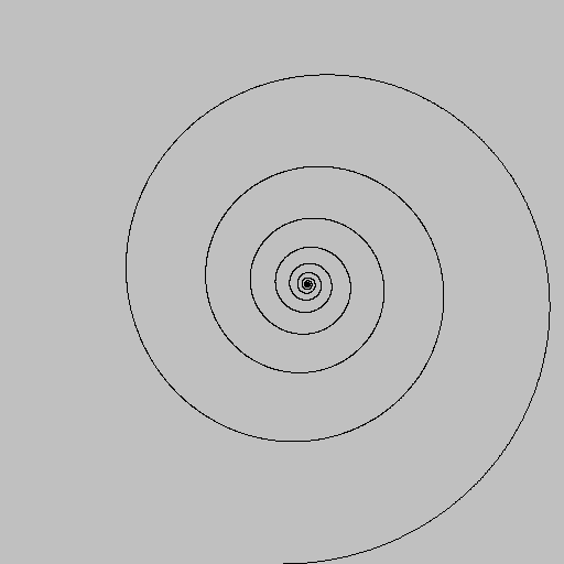
The logarithmic spiral was first described by Rene Descartes in 1638. Jacob Bernoulli was so amazed by its mathematical properties that he named it the spira mirabilis (miraculous spiral). Many people also consider it to be "miraculous" that this precise curve is clearly present in a broad variety of natural phenomena:
Nautilus Shell Spiral Galaxy Storm Clouds


Brownian motion.
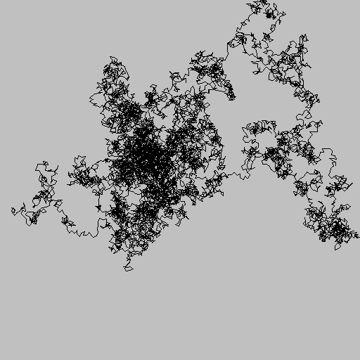
Imagine a disoriented turtle (again following its standard alternating turn and step regimen) turns in a random direction before each step. The program drunk.py plots the path followed by such a turtle. In 1827, the botanist Robert Brown observed through a microscope that pollen grains immersed in water seemed to move about in just such a random fashion, which later became known as Brownian motion and led to Albert Einstein's insights into the atomic nature of matter.
% python drunk.py 10000 .01
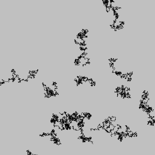
The program drunks.py plots many such turtles, all of whom wander around.
% python drunks.py 20 500 .005% python drunks.py 20 1000 .005% python drunks.py 20 5000 .005


Turtle graphics was originally developed by Seymour Papert at MIT in the 1960s as part of an educational programming language, Logo. But turtle graphics is no toy, as we have just seen in numerous scientific examples. Turtle graphics also has numerous commercial applications. For example, it is the basis for PostScript, a programming language for creating printed pages that is used for most newspapers, magazines, and books.
Complex Numbers
A complex number is a number of the form x + yi, where x and y are real numbers and i is the square root of -1. The number x is known as the real part of the complex number, and the number y is known as the imaginary part. This terminology stems from the idea that the square root of -1 has to be an imaginary number, because no real number can have this value. Complex numbers are a quintessential mathematical abstraction: whether or not one believes that it makes sense physically to take the square root of -1, complex numbers help us understand the natural world.
The Python language provides a complex (with a lowercase c) data type. In real applications you certainly should take advantage of complex unless you find yourself wanting more operations than it provides. However, since developing a data type for complex numbers is a prototypical exercise in object-oriented programming, we now consider our own Complex (with an uppercase C) data type. Doing so will allow us to consider a number of interesting issues surrounding data types for mathematical abstractions, in a nontrivial setting.
The operations on complex numbers that are needed for basic computations are to add and multiply them by applying the commutative, associative, and distributive laws of algebra (along with the identity i2 = -1); to compute the magnitude; and to extract the real and imaginary parts, according to the following equations:
- Addition: (x+yi) + (v+wi) = (x+v) + (y+w)i
- Multiplication: (x + yi) * (v + wi) = (xv - yw) + (yv + xw)i
- Magnitude: |x + yi| = (x2 + y2)1/2
- Real part: Re(x + yi) = x
- Imaginary part: Im(x + yi) = y
As usual, we start with an API that specifies the data-type operations.
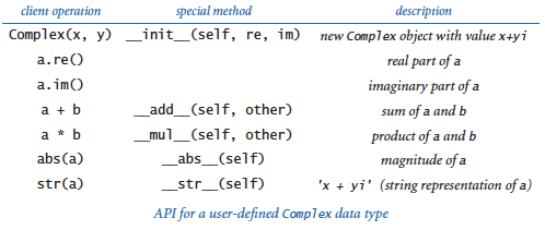
The Complex class defined in complex.py implements that API.
Special methods.
When Python sees the expressiona + b in client code, it replaces it with the method call a.__add__(b). Similarly, Python replaces a * b with the method call a.__mul__(b). Therefore, we need only to implement the special methods __add__() and __mul__() for addition and multiplication to operate as expected. The mechanism is the same one that we used to support Python's built-in str() function for Charge, by implementing the __str__() special method, except that the special methods for arithmetic operators take two arguments. The above API includes an extra column that maps the client operations to the special methods. We generally omit this column in our APIs because these names are standard, and irrelevant to clients. The list of Python special methods is extensive — we will discuss them further in Section 3.3.
Accessing instance variables in objects of this type.
The implementations of both__add__() and __mul__() need to access values in two objects: the object passed as an argument and the object used to call the method (that is, the object referenced by self). When the client calls a.__add__(b), the parameter variable self is set to reference the same object as argument a does, and the parameter variable other is set to reference the same object as argument b does. We can access the instance variables of a using self._re and self._im, as usual. To access the instance variables of b, we use the code other._re and other._im. Since our convention is to keep the instance variables private, we do not access directly instance variables in another class. Accessing instance variables within another object in the same class does not violate this privacy policy.
Immutability.
The two instance variables inComplex are set for each Complex object when it is created and do not change during the lifetime of an object. That is, Complex objects are immutable.
Mandelbrot Set.
The Mandelbrot set is a specific set of complex numbers discovered by Benoit Mandelbrot that has many fascinating properties. It is a fractal pattern that is related to the Barnsley fern, the Sierpinski triangle, the Brownian bridge, the Koch curve, the drunken turtle, and other recursive (self-similar) patterns and programs that we have seen in this book. The set of points in the Mandelbrot set cannot be described by a single mathematical equation. Instead, it is defined by an algorithm and, therefore, a perfect candidate for a complex client: we study the set by composing a program to plot it.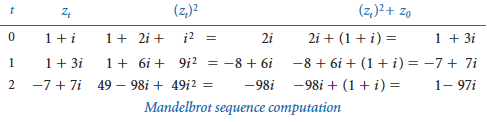
Now, if the sequence |zt| diverges to infinity, then z0 is not in the Mandelbrot set; if the sequence is bounded, then z0 is in the Mandelbrot set.
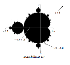
To visualize the Mandelbrot set, we sample complex points, just as we sample real-valued points to plot a real-valued function. Each complex number x + yi corresponds to a point (x, y) in the plane, so we can plot the results as follows: for a specified resolution n, we define a regularly spaced n-by-n pixel grid within a specified square and draw a black pixel if the corresponding point is in the Mandelbrot set and a white pixel if it is not.
There is no simple test that enables us to conclude that a point is surely in the set. But there is a simple mathematical test that tells us for sure that a point is not in the set: if the magnitude of any number in the sequence ever exceeds 2 (such as 1 + 3i), then the sequence surely will diverge. The program mandelbrot.py uses this test to plot a visual representation of the Mandelbrot set. Since our knowledge of the set is not quite black-and-white, we use grayscale in our visual representation. The basis of the computation is the function mandel(), which takes a complex argument z0 and an integer argument limit and computes the Mandelbrot iteration sequence starting at z0, returning the number of iterations for which the magnitude stays less than (or equal to) 2, up to the given limit. The complexity of the images that this simple program produces is remarkable, even when we zoom in on a tiny portion of the plane.
% python mandelbrot.py 512 -.5 0 2% python mandelbrot.py 512 .1015 -.633 .01


Producing an image with mandelbrot.py requires hundreds of millions of operations on complex values. Accordingly, we use Python's complex data type, which is certain to be more efficient than the Complex data type that we just considered.
Commercial Data Processing
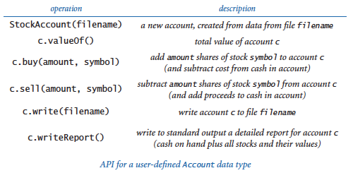
Suppose that a stock broker needs to maintain customer accounts containing shares of various stocks. That is, the set of values the broker needs to process includes the customer's name, number of different stocks held, number of shares and ticker symbol for each stock, and cash on hand. To process an account, the broker needs at least the operations defined in this API:
The customer information has a long lifetime and needs to be saved in a file or database. To process an account, a client program needs to read information from the corresponding file; process the information as appropriate; and, if the information changes, write it back to the file, saving it for later. To enable this kind of processing, we need a file format and an internal representation, or a data structure, for the account information.
File format.
Modern systems often use text files, even for data, to minimize dependence on formats defined by any one program. For simplicity, we use a direct representation where we list the account holder's name (a string), cash balance (a float), and number of stocks held (an integer), followed by a line for each stock giving the number of shares and the ticker symbol. For example the file turing.txt contains these data:
Data structure.
To implement aStockAccount, we use the following instance variables:
- A string for the account name
- A float for the cash on hand
- An integer for the number of stocks
- An array of strings for stock symbols
- An array of integers for numbers of shares
The StockAccount class defined in stockaccount.py implements those design decisions. The arrays _stocks[] and _shares[] are known as parallel arrays. Given an index i, _stocks[i] gives a stock symbol and _shares[i] gives the number of shares of that stock in the account. The valueOf() method uses stockquote.py (from Section 3.1) to get each stock's price from the web. The implementations of buy() and sell() require the use of basic mechanisms introduced in Section 4.4, so we defer them to an exercise in that section. The test client accepts a the name of a file (such as the aforementioned turing.txt) as a command-line argument, and writes an appropriate report.
Q & A
Q. Can I define a class in a file whose name is unrelated to the class name? Can I define more than one class in a single .py file?
A. Yes and yes, but we do not do so in this chapter as a matter of style. In Chapter 4, we will encounter a few situations where these features are appropriate.
Q. If __init__() is technically not a constructor, what is?
A. Another special function, __new__(). To create a object, Python first calls __new__() and then __init__(). For the programs in this book, the default implementation of __new__() serves our purposes, so we do not discuss it.
Q. Must every class have a constructor?
A. Yes, but if you do not define a constructor, Python provides a default (no-argument) constructor automatically. With our conventions, such a data type would be useless, as it would have no instance variables.
Q. Why do I need to use self explicitly when referring to instance variables?
A. Syntactically, Python needs some way to know whether you are assigning to a local variable or to an instance variable. In many other programming languages (such as C++ and Java), you declare explicitly the data type's instance variables, so there is no ambiguity. The self variable also makes it easy for programmers to know whether code is referring to a local variable or an instance variable.
Q. Suppose I do not include a __str__() method in my data type. What happens if I call str() or stdio.writeln() with an object of that type?
A. Python provides a default implementation that returns a string containing the object's type and its identity (memory address). This is unlikely to be of much use, so you usually want to define your own.
Q. Are there other kinds of variables besides parameter, local, and instance variables in a class?
A. Yes. Recall from Chapter 1 that you can define global variables in global code, outside of the definition of any function, class, or method. The scope of global variables is the entire .py file. In modern programming, we focus on limiting scope and therefore rarely use global variables (except in tiny scripts not intended for reuse). Python also supports class variables, which are defined inside a class but outside any method. Each class variable is shared among all of the objects in a class; this contrasts with instance variables, where there is one per object. Class variables have some specialized uses, but we do not use them in this book.
Q. Is it just me, or are Python's conventions for naming things complicated?
A. Yes, but this is also true of many other programming languages. Here is a quick summary of the naming conventions we have encountered in the book:
- A variable name starts with lowercase letter.
- A constant variable name consists of uppercase letters.
- An instance variable name starts with an underscore and a lowercase letter.
- A method name starts with a lowercase letter.
- A special method name starts with a double underscore and a lowercase letter and ends with a double underscore.
- A user-defined class name starts with an uppercase letter.
- A built-in class name starts with a lowercase letter.
- A script or module is stored in a file whose name consists of lowercase letters and ends with
.py.
Most of those conventions are not part of the language, though many Python programmers treat them as if they are. You might wonder: If they are so important, why not make them part of the language? Good question. Still, some programmers are passionate about such conventions, and you are likely to someday encounter a teacher, supervisor, or colleague who insists that you follow a certain style, so you may as well go with the flow. Indeed, many Python programmers separate multi-word variable names with underscores instead of capital letters, preferring is_prime and hurst_exponent to isPrime and hurstExponent.
Q. How can I specify a literal for the complex data type?
A. Appending the character j to a numeric literal produces an imaginary number (whose real part is zero). You can add this character to a numeric literal to produce a complex number, as in 3 + 7j. The choice of j instead of i is common in some engineering disciplines. Note that j is not a complex literal — instead, you must use 1j.
Q. The mandelbrot.py program creates a huge number of complex objects. Doesn't all that object-creation overhead slow things down?
A. Yes, but not so much that we cannot generate our plots. Our goal is to make our programs readable and easy to compose and maintain. Limiting scope via the complex number abstraction helps us achieve that goal. If you need to speed up mandelbrot.py significantly for some reason, you might consider bypassing the complex number abstraction and using a lower-level language where numbers are not objects. Generally, Python is not optimized for performance. We will revisit this issue in Chapter 4.
Q. Why is it okay for the __add__(self, other) method in complex.py to refer to the instance variables of the parameter variable other? Aren't these instance variables supposed to be private?
A. Python programmers view privacy as relative to a particular class, not to a particular object. So, a method can refer to the instance variables of any object in the same class. Python has no "superprivate" naming conventions in which you can refer only to the instance variables of the invoking object. Accessing the instance variables of other can be a bit risky, however, because a careless client might pass an argument that is not of type Complex, in which case we would be (unknowingly) accessing an instance variable in another class! With a mutable type, we might even (unknowingly) modify or create instance variables in another class!
Q. If methods are really functions, can I call a method using function-call syntax?
A. Yes, you can call a function defined in a class as either a method or an ordinary function. For example, if c is an object of type Charge, then the function call Charge.potentialAt(c, x, y) is equivalent to the method call c.potentialAt(x, y). In object-oriented programming, we prefer the method-call syntax to highlight the role of the featured object and to avoid hardwiring the name of the class into the function call.
Exercises
-
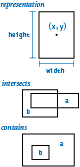
Consider the data-type implementation for (axis-aligned) rectangles shown below, which represents each rectangle with the coordinates of its center point and its width and height. Compose an API for this data type, and fill in the code for
perimeter(),intersects(),contains(), anddraw(). Note: Treat coincident lines as intersecting, so that, for example,a.intersects(a)is True anda.contains(a)is True.class Rectangle: # Construct self with center (x, y), width w, and height h. def __init__(self, x, y, w, h): self._x = x self._y = y self._width = w; self._height = h; # Return the area of self. def area(self): return self._width * self._height # Return the perimeter of self. def perimeter(self): ... # Return True if self intersects other, and False otherwise. def intersects(self, other): ... # Return True if other is completely inside of self, and False # otherwise. def contains(self, other): ... # Draw self on stddraw. def draw(self): ... -
Compose a test client for
Rectanglethat takes three command-line argumentsn,lo, andhi; generatesnrandom rectangles whose width and height are uniformly distributed betweenloandhiin the unit square; draws those rectangles to standard drawing; and writes their average area and average perimeter to standard output. -
Add code to your test client from the previous exercise code to compute the average number of pairs of rectangles that intersect and are contained in one another.
-
Develop an implementation of your
RectangleAPI from the previous exercises that represents rectangles with the coordinates of their lower left and upper right corners. Do not change the API. -
Create a data type
Locationthat represents a location on Earth using latitudes and longitudes. Include a methoddistanceTo()that computes distances using the great-circle distance (see the Great circle exercise in Section 1.2). -
Python provides a data type
Fraction, defined in the standard modulefractions.py, that implements rational numbers. Implement your own version of that data type. Specifically, develop an implementation of the following API for a data type for rational numbers: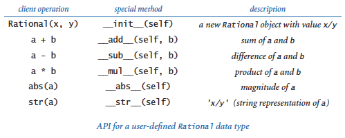
Use
euclid.gcd()defined in euclid.py (from Section 2.3) to ensure that the numerator and denominator never have any common factors. Include a test client that exercises all of your methods. -
An interval is defined to be the set of all points on a line greater than or equal to
leftand less than or equal toright. In particular, an interval withrightless thanleftis empty. Compose a data typeIntervalthat implements the API shown below. Include a test client that is a filter and takes a floatxfrom the command line and writes to standard output (1) all of the intervals from standard input (each defined by a pair of floats) that containxand (2) all pairs of intervals from standard input that intersect one another.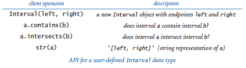
-
Develop an implementation of your
RectangleAPI (from a previous exercise in this section) that takes advantage ofInterval(from the previous exercise in this section) to simplify and clarify the code. -
Compose a data type
Pointthat implements the following API. Include a client of your own design.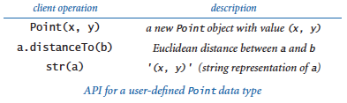
-
Add methods to
Stopwatch, as defined in stopwatch.py that allow clients to stop and restart the stopwatch. -
Use a
Stopwatchto compare the cost of computing harmonic numbers with aforloop (as shown in Section 1.3) as opposed to using the recursive method given in Section 2.3. -
Modify the test client in turtle.py to produce stars with
npoints for oddn. -
Compose a version of mandelbrot.py that uses
Complexinstead of Python'scomplex. Then useStopwatch(as defined in stopwatch.py) to compute the ratio of the running times of the two programs. -
Modify the
__str__()method in classComplex, as defined in complex.py, so that it writes complex numbers in the traditional format. For example, it should write the value 3 - i as3 - iinstead of3.0 + -1.0i, the value 3 as3instead of3.0 + 0.0i, and the value 3i as3iinstead of0.0 + 3.0i. -
Compose a
Complexclient that takes three floats a, b, and c as command-line arguments and writes the complex roots of ax2 + bx + c. -
Write a
ComplexclientRootsthat takes two floats a and b and an integer n from the command line and writes the nth roots of a + bi. Note: skip this exercise if you are not familiar with the operation of taking roots of complex numbers. -
Implement the following additions to the
ComplexAPI: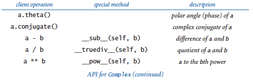
Include a test client that exercises all of your methods.
-
Find a
complexnumber for whichmandel()(from mandelbrot.py) returns a number greater than 100, and then zoom in on that number.
What is wrong with the following code?
class Charge:
    def __init__(self, x0, y0, q0):
        _rx = x0  # Position
        _ry = y0  # Position
        _q = q0   # Charge
...
Solution. The assignment statements in the constructor create local variables _rx, _ry, and _q, which are assigned values from the parameter variables but are never used. They disappear when the constructor is finished executing. Instead, the constructor should create instance variables by prefixing each variable with self followed by the dot operator, like this:
class Charge:
    def __init__(self, x0, y0, q0):
        self._rx = x0  # Position
        self._ry = y0  # Position
        self._q = q0   # Charge
...
The underscore is not strictly required in Python, but we follow this standard Python convention throughout this book to indicate that our intent is for instance variables to be private.
Creative Exercises
-
Mutable charges. Modify the
Chargeclass as defined in charge.py so that the charge valueq0can change, by adding a methodincreaseCharge()that takes a float argument and adds the given value toq0. Then, compose a client that initializes an array with:a = stdarray.create1D(3) a[0] = Charge(.4, .6, 50) a[1] = Charge(.5, .5, -5) a[2] = Charge(.6, .6, 50)
and then displays the result of slowly decreasing the charge value of
a[1]by wrapping the code that computes the picture in a loop like the following:for t in range(100): # Compute the picture p. stddraw.clear() stddraw.picture(p) stddraw.show(0) a[1].increaseCharge(-2.0) -
Complex timing. Compose a
Stopwatchclient (see stopwatch.py) that compares the cost of usingcomplexto the cost of composing code that directly manipulates two float values, for the task of doing the calculations in mandelbrot.py. Specifically, create a version of mandelbrot.py that just does the calculations (remove the code that refers toPicture), then create a version of that program that does not usecomplex, and then compute the ratio of the running times. -
Quaternions. In 1843, Sir William Hamilton discovered an extension to complex numbers called quaternions. A quaternion is a vector a = (a0, a1, a2, a3) with the following operations:
- Magnitude: |a| = (a02 + a12 + a22 + a32)1/2.
- Conjugate: the conjugate of a is (a0, -a1, -a2, -a3).
- Inverse: a-1 = (a0 /|a|, -a1 /|a|, -a2 /|a|, -a3 /|a|).
- Sum: a + b = (a0 + b0, a1 + b1, a2 + b2, a3 + b3).
- Product: a * b = (a0 b0 - a1 b1 - a2 b2 - a3 b3, a0 b1 - a1 b0 + a2 b3 - a3 b2, a0 b2 - a1 b3 + a2 b0 + a3 b1, a0 b3 + a1 b2 - a2 b1 + a3 b0).
- Quotient: a / b = ab-1.
Create a data type for quaternions and a test client that exercises all of your code. Quaternions extend the concept of rotation in three dimensions to four dimensions. They are used in computer graphics, control theory, signal processing, and orbital mechanics.
Dragon curves. Compose a recursive client of
Turtle(as defined in turtle.py) nameddragon.pythat draws dragon curves (see the exercises in Sections 1.2 and 1.5). These curves, originally discovered by three NASA physicists, were popularized in the 1960s by Martin Gardner and later used by Michael Crichton in the book and movie Jurassic Park. This exercise can be solved with remarkably compact code, based on a pair of mutually interacting recursive functions derived directly from the definition in the exercise in Section 1.2. One of them,dragon(), should draw the curve as you expect; the other,nogard(), should draw the curve in reverse order.


-
Hilbert curves. A space-filling curve is a continuous curve in the unit square that passes through every point. Compose a recursive client of
Turtle(as defined in turtle.py) that produces these recursive patterns, which approach a space-filling curve that was defined by the mathematician David Hilbert at the end of the 19th century. See the previous exercise. You need a pair of methods:hilbert(), which traverses a Hilbert curve, andtreblih(), which traverses a Hilbert curve in reverse order.


-
Gosper island. Compose a recursive client of
Turtle(as defined in turtle.py) that produces these recursive patterns.


-
Data analysis. Compose a data type for use in running experiments where the control variable is an integer in the range [0, n) and the dependent variable is a float. For example, studying the running time of a program that takes an integer argument would involve such experiments. A Tukey plot is a way to visualize the statistics of such data (see the Tukey plot exercise in Section 2.2). Implement the following API:
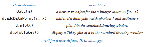
You can use the functions in
stdstatsto do the statistical calculations and draw the plots. Usestddrawso clients can use different colors forplot()andtukeyPlot()(for example, light gray for all the points and black for the Tukey plot). Compose a test client that plots the results (percolation probability) of running experiments with percolation.py (from Section 2.4) as the grid size increases. -
Elements. Compose a data type
Elementfor entries in the periodic table of elements. Include data type values for element, atomic number, symbol, and atomic weight and accessor methods for each of these values. Then, create a data typePeriodicTablethat reads values from a file to create an array ofElementobjects and responds to queries on standard input so that a user can type a molecular equation likeH2Oand the program responds by printing the molecular weight. Develop APIs and implementations for each data type.The file elements.csv contains the data that the program should read. Include fields for element, atomic number, symbol, and atomic weight. (Ignore fields for boiling point, melting point, density (kg/m3), heat vapour (
kJ/mol), heat fusion (kJ/mol), thermal conductivity (W/m/K), and specific heat capacity (J/kg/K) since it's not known for all elements). The file is in CSV format (fields separated by commas). -
Stock prices. The file djia.csv contains all closing stock prices in the history of the Dow Jones Industrial Average, in the comma-separated value format. Compose a data type
Entrythat can hold one entry in the table, with values for date, opening price, daily high, daily low, closing price, and so forth. Then, compose a data typeTablethat reads the file to build an array ofEntryobjects and supports methods for computing averages over various periods of time. Finally, create interestingTableclients to produce plots of the data. Be creative: this path is well-trodden. -
Chaos with Newton's method. The polynomial f(z) = z4 - 1 has four roots: at 1, -1, i, and -i. We can find the roots using Newton's method in the complex plane: zk+1 = zk - f(zk)/f'(zk). Here, f(z) = z4 - 1 and f'(z) = 4z3. The method converges to one of the four roots, depending on the starting point z0. Compose a client of
Complex(as defined in complex.py) namedNewtonthat takes a command-line argument n and colors pixels in an n-by-nPicturewhite, red, green, or blue by mapping the pixels complex points in a regularly spaced grid in the square of size 2 centered at the origin and coloring each pixel according to which of the four roots the corresponding point converges (black if no convergence after 100 iterations).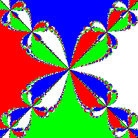
-
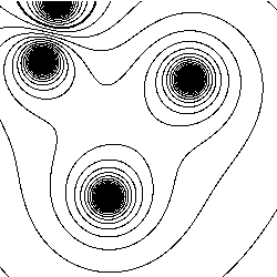
Equipotential surfaces. An equipotential surface is the set of all points that have the same electric potential V. Given a group of point charges, it is useful to visualize the electric potential by plotting equipotential surfaces (also known as a contour plot). Compose a program
equipotential.pythat draws a line every 5V by computing the potential at each pixel and checking whether the potential at the corresponding point is within 1 pixel of a multiple of 5V. Note: A very easy approximate solution to this exercise is obtained from potential.py (from Section 3.1) by scrambling the color values assigned to each pixel, rather than having them be proportional to the grayscale value. For example, the accompanying figures are created by inserting the code above it before creating theColor. Explain why it works, and experiment with your own version.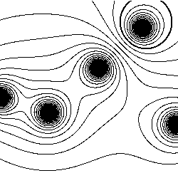
-
Color Mandelbrot plot. Create a file of 256 integer triples that represent interesting
Colorvalues, and then use those colors instead of grayscale values to plot each pixel in mandelbrot.py. Read the values to create an array of 256Colorvalues, then index into that array with the return value ofmandel(). By experimenting with various color choices at various places in the set, you can produce astonishing images. mandel.txt is an example.% python mandelbrot.py -1.5 -1.0 2.0 2.0% python mandelbrot.py 0.10259 -0.641 0.0086 0.0086

-
Julia sets. The Julia set for a given complex number c is a set of points related to the Mandelbrot function. Instead of fixing z and varying c, we fix c and vary z. Those points z for which the modified Mandelbrot function stays bounded are in the Julia set; those for which the sequence diverges to infinity are not in the set. All points z of interest lie in the 4-by-4 box centered at the origin. The Julia set for c is connected if and only if c is in the Mandelbrot set! Compose a program
colorjulia.pythat takes two command line arguments a and b, and plots a color version of the Julia set for c = a + bi, using the color-table method described in the previous exercise.python colorjulia.py -1.25 0.00python colorjulia.py-0.75 0.10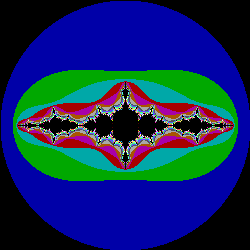

-
Biggest winner and biggest loser. Compose a client of
StockAccount(as defined in stockaccount.py) that builds an array ofStockAccountobjects, computes the total value of each account, and writes a report for the account with the largest value and the account with the smallest value. Assume that the information in the accounts are kept in a single file that contains the information for each of the accounts, one after the other, in the format given described earlier in this page.