A Case Study: Small World Phenomenon

4.5 A Case Study: Small World Phenomenon

The mathematical model that we use for studying the nature of pairwise connections among entities is known as the graph. Graphs are important for studying the natural world and for helping us to better understand and refine the networks that we create.

Some graphs exhibit a specific property known as the small-world phenomenon. You may be familiar with this property, which is sometimes known as six degrees of separation. It is the basic idea that, even though each of us has relatively few acquaintances, there is a relatively short chain of acquaintances (the six degrees of separation) separating us from one another. Scientists are interested in small-world graphs because they model natural phenomena, and engineers are interested in building networks that take advantage of the natural properties of small-world graphs.

In this section, we address basic computational questions surrounding the study of small-world graphs.

Graph Data Type

We begin with some basic definitions. A graph is composed of a set of vertices and a set of edges. Each edge represents a connection between two vertices. Two vertices are neighbors if they are connected by an edge, and the degree of a vertex is its number of neighbors.

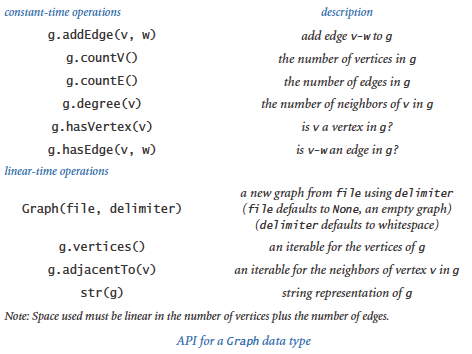
Graph-processing algorithms generally first build an internal representation of a graph by adding edges, then process it by iterating through the vertices and through the edges that are adjacent to a vertex. This API supports such processing.

The program graph.py implements this API. Its internal representation is a symbol table of sets: the keys are vertices and the values are the sets of neighbors — the vertices adjacent to the key. A small example is illustrated at right. To implement this representation, we use the two built-in data types dict and set that we introduced in Section 4.4.

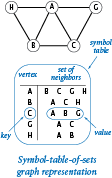
A natural way to write a Graph is to put the vertices one per line, each followed by a list of its immediate neighbors. Accordingly, we support the built-in function str() by implementing __str__() as shown in graph.py. The resulting string includes two representations of each edge, one for the case in which we discover that w is a neighbor of v and one for the case in which we discover that v is a neighbor of w. Many graph algorithms are based on this basic paradigm of processing each edge in the graph (twice). This implementation is intended for use only for small graphs, as the running time is quadratic in the string length on some systems.

The output format for str() also defines a reasonable input file format. The __init__() method supports creating a graph from a file in this format (each line is a vertex name followed by the names of neighbors of that vertex, separated by whitespace). For flexibility, we allow for the use of delimiters besides whitespace (so that, for example, vertex names may contain spaces), as shown in graph.py.

Graph Client Example

As a first graph-processing client, we consider an example of social relationships — one that is certainly familiar to you and for which extensive data is readily available.

On this booksite you can find the file movies.txt which contains a list of movies and the performers who appeared in them. Each line gives the name of a movie followed by the cast (a list of the names of the performers who appeared in that movie). Since names have spaces and commas in them, we use the '/' character as a delimiter.

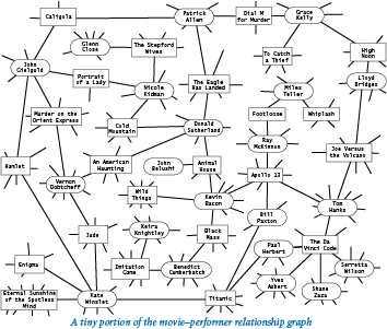
Using Graph, we can compose a simple and convenient client for extracting information from movies.txt. We begin by building a Graph to better structure the information. What should the vertices and edges model? We choose to have vertices for both the movies and the performers, with an edge connecting each movie to each performer in that movie. As you will see, programs that process this graph can answer a great variety of interesting questions for us.

The program invert.py is a first example. It is a Graph client that takes a query, such as the name of a movie, and writes the list of performers who appear in that movie. A more interesting feature of invert.py is that you can type the name of a performer and get the list of movies in which that performer has appeared. Why does this work? Even though the database seems to connect movies to performers and not the other way around, the edges in the graph are connections that also connect performers to movies.

A graph in which connections all connect one kind of vertex to another kind of vertex is known as a bipartite graph. As this example illustrates, bipartite graphs have many natural properties that we can often exploit in interesting ways.

It is worth reflecting on the fact that building a bipartite graph provides a simple way to automatically invert any index! This inverted-index functionality is a direct benefit of the graph data structure. Next, we examine some of the added benefits to be derived from algorithms that process the data structure.

Shortest Paths in Graphs

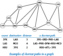
Given two vertices in a graph, a path is a sequence of vertices connected by edges. A shortest path is one with the minimal number of edges over all such paths (there may be multiple shortest paths). Finding a shortest path connecting two vertices in a graph is a fundamental problem in computer science.

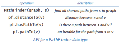
Depending on the application, clients have various needs with regard to shortest paths. Our choice is to start with the following API:

In huge graphs or for huge numbers of queries, we have to pay particular attention to API design because the cost of computing paths might prove to be prohibitive. With this design, clients can create a PathFinder object for a given graph and a given vertex, and then use that object either to find the length of the shortest path or to iterate over the vertices on a shortest path to any other vertex in the graph. An implementation of these methods is known as a single-source shortest-path algorithm. A classic algorithm known as breadth-first search provides a direct and elegant solution where the constructor takes linear time, distanceTo() takes constant time, and pathTo() takes time proportional to the length of the path. Before examining our implementation, we will consider some clients.

Single-source client.

Suppose that you have available to you the graph of vertices and connections for your no-frills airline's route map. Then, using your home city as a source, you can compose a client that writes your route anytime you want to go on a trip. The program separation.py is a PathFinder client that provides this functionality for any graph. You are encouraged to explore the properties of shortest paths by running PathFinder on our sample input routes.txt or any input model that you choose.

Degrees of separation.

One of the classic applications of shortest-paths algorithms is to find the degrees of separation of individuals in social networks. To fix ideas, we discuss this application in terms of a recently popularized pastime known as the Kevin Bacon game, which uses the movie-performer graph that we just considered. Kevin Bacon is a prolific actor who appeared in many movies. We assign every performer who has appeared in a movie a Bacon number: Bacon himself is 0, any performer who has been in the same cast as Bacon has a Kevin Bacon number of 1, any other performer (except Bacon) who has been in the same cast as a performer whose number is 1 has a Kevin Bacon number of 2, and so forth. For example, Meryl Streep has a Kevin Bacon number of 1 because she appeared in The River Wild with Kevin Bacon. Nicole Kidman's number is 2: although she did not appear in any movie with Kevin Bacon, she was in Cold Mountain with Donald Sutherland, and Sutherland appeared in Animal House with Kevin Bacon. Given the name of a performer, the simplest version of the game is to find some alternating sequence of movies and performers that lead back to Kevin Bacon. Remarkably, pathfinder.py is precisely the program that you need to find a shortest path that establishes the Bacon number of any performer in movies.txt: the Bacon number of any performer is precisely half the distance between Kevin Bacon and that performer.

Shortest-path distances.

We define the distance between two vertices to be the length of the shortest path between them. The first step in understanding breadth-first search is to consider the problem of computing distances between the source and each vertex (the implementation of distanceTo() in PathFinder). Our approach is to compute and store away all the distances in the constructor, and then just return the requested value when a client invokes distanceTo(). To associate an integer distance with each vertex name, we use a symbol table:

_distTo = dict()

The purpose of this symbol table is to associate with each vertex the length of the shortest path (the distance) between that vertex and s. To do that we consider the vertices in order of their distance from s, ignoring vertices whose distance to s is already known. To organize the computation, we use a FIFO queue. Starting with s on the queue, we perform the following operations until the queue is empty:

Dequeue a vertex v.
Assign all of v's unknown neighbors a distance 1 greater than v's distance.
Enqueue all of the unknown neighbors.

This method dequeues the vertices in nondecreasing order of their distance from the source s.

Shortest-paths tree.

We need not only distances from the source, but also paths. To implement pathTo(), we use a subgraph known as the shortest-paths tree, defined as follows:

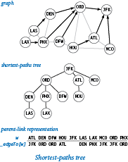
Put the source vertex s at the root of the tree.
Put vertex v's neighbors in the tree if they are added to the queue, with an edge connecting each to v.

Since we enqueue each vertex only once, this structure is a proper tree: it consists of a root (the source) connected to one subtree for each neighbor of the source. Studying such a tree, you can see immediately that the distance from each vertex to the root in the tree is the same as the shortest-path distance to the source in the graph. More importantly, each path in the tree is a shortest path in the graph. This observation is important because it gives us an easy way to provide clients with the shortest paths themselves (implement pathTo() in PathFinder).

First, we maintain a symbol table associating each vertex with the vertex one step nearer to the source on the shortest path:

_edgeTo = dict()

To each vertex w, we want to associate the previous stop on the shortest path from the source to w. Augmenting the shortest-distances method to also compute this information is easy: when we enqueue w because we first discover it as a neighbor of v, we do so precisely because v is the previous stop on the shortest path from the source to w, so we can assign _edgeTo[w] = v. The _edgeTo data structure is nothing more than a representation of the shortest-paths tree: it provides a link from each node to its parent in the tree. Then, to respond to a client request for the path from the source to v (a call to pathTo(v) in PathFinder), we follow these links up the tree from v, which traverses the path in reverse order. We collect the vertices in an array as we encounter them, then reverse the array, so the client gets the path from s to v when using the iterator returned from pathTo().

Breadth-first search.

This process is known as breadth-first search because it searches broadly in the graph. By contrast, another important graph-search method known as depth-first search is based on a recursive method like the one we used in percolation.py from Section 2.4 and searches deeply into the graph. Depth-first search tends to find long paths; breadth-first search is guaranteed to find shortest paths.

Small-World Graphs

Scientists have identified a particularly interesting class of graphs that arise in numerous applications in the natural and social sciences. Small-world graphs are characterized by the following three properties:

They are sparse: the number of vertices is much smaller than the number of edges.
They have short average path lengths: if you pick two random vertices, the length of the shortest path between them is short.
They exhibit local clustering: if two vertices are neighbors of a third vertex, then the two vertices are likely to be neighbors of each other.

We refer to graphs having these three properties collectively as exhibiting the small-world phenomenon. The term small world refers to the idea that the preponderance of vertices have both local clustering and short paths to other vertices. The modifier phenomenon refers to the unexpected fact that so many graphs that arise in practice are sparse, exhibit local clustering, and have short paths.

A key question in such research is the following: Given a graph, how can we tell whether it is a small-world graph? To answer this question, we begin by imposing the conditions that the graph is not small (say, 1000 vertices or more) and that it is connected (there exists some path connecting each pair of vertices). Then, we need to settle on specific thresholds for each of the small-world properties:

By sparse, we mean the average vertex degree is less than 20 lg V.
By short average path length, we mean the average length of the shortest path between two vertices is less than 10 lg V.
By locally clustered, we mean that a certain quantity known as the clustering coefficient should be greater than 10%.

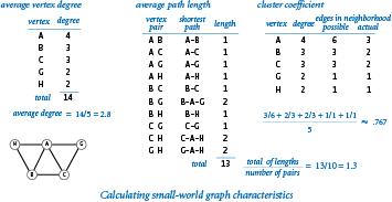
The definition of locally clustered is a bit more complicated than the definitions of sparsity and average path length. Intuitively, the clustering coefficient of a vertex represents the probability that if you pick two of its neighbors at random, they will also be connected by an edge. More precisely, if a vertex has t neighbors, then there are t(t-1)/2 possible edges that connect those neighbors; its local clustering coefficient is the fraction of those edges that are in the graph (or 0 if the vertex has degree 0 or 1). The clustering coefficient of a graph is the average of the local clustering coefficients of its vertices. If that average is greater than 10%, we say that the graph is locally clustered. The diagram below calculates these three quantities for a tiny graph.

To better familiarize you with these definitions, we next define some simple graph models, and consider whether they describe small-world graphs by checking whether they exhibit the three requisite properties.

Complete graphs.

A complete graph with V vertices has V (V-1) / 2 edges, one connecting each pair of vertices. Complete graphs are not small-world graphs. They have short average path length (every shortest path has length is 1) and they exhibit local clustering (the cluster coefficient is 1), but they are not sparse (the average vertex degree is V-1, which is much greater than 20 lg V for large V).

Ring graphs.

A ring graph is a set of V vertices equally spaced on the circumference of a circle, with each vertex connected to its neighbor on either side. In a k-ring graph, each vertex is connected to its k nearest neighbors on either side. The diagram at right illustrates a 2-ring graph with 16 vertices. Ring graphs are also not small-world graphs. For example, 2-ring graphs are sparse (every vertex has degree 4) and exhibit local clustering (the cluster coefficient is 1/2), but their average path length is not short.

Random graphs.

The Erdos-Renyi model is a well studied model for generating random graphs. In this model, we build a random graph on V vertices by including each possible edge with probability p. Random graphs with a sufficient number of edges are very likely to be connected and have short average path lengths but they are not small-world graphs, because they are not locally clustered.

These examples illustrate that developing a graph model that satisfies all three properties simultaneously is a puzzling challenge. Take a moment to try to design a graph model that you think might do so. After you have thought about this problem, you will realize that you are likely to need a program to help with calculations. Also, you may agree that it is quite surprising that they are found so often in practice. Indeed, you might be wondering if any graph is a small-world graph!

Choosing 10% for the clustering threshold instead of some other fixed percentage is somewhat arbitrary, as is the choice of 20 lg V for the sparsity threshold and 10 lg V for the short paths threshold, but we often do not come close to these borderline values. For example, consider the web graph, which has a vertex for each web page and an edge connecting two web pages if they are connected by a link. Scientists estimate that the number of clicks to get from one web page to another is rarely more than about 30. Since there are billions of web pages, this estimate implies that the average length of a path between two vertices is very short, much lower than our 10 lg V threshold (which would be about 300 for 1 billion vertices).

Having settled on the definitions, testing whether a graph is a small-world graph can still be a significant computational burden. As you probably have suspected, the graph-processing data types that we have been considering provide precisely the tools that we need. The program smallworld.py is a Graph and PathFinder client that implements these tests. Without the efficient data structures and algorithms that we have been considering, the cost of this computation would be prohibitive. Even so, for large graphs (such as movies.txt), we must resort to statistical sampling to estimate the average path length and the cluster coefficient in a reasonable amount of time because the functions averagePathLength() and clusteringCoefficient() take quadratic time.

A classic small-world graph.

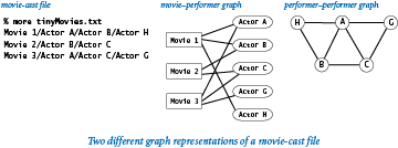
Our movie-performer graph is not a small-world graph, because it is bipartite and therefore has a clustering coefficient of 0. Also, some pairs of performers are not connected to each other by any paths. However, the simpler performer-performer graph defined by connecting two performers by an edge if they appeared in the same movie is a classic example of a small-world graph (after discarding performers not connected to Kevin Bacon). The diagram below illustrates the movie-performer and performer-performer graphs associated with a tiny movie-cast file.

The program performer.py is a script that creates a performer-performer graph from a file in our movie-cast input format. Recall that each line in a movie-cast file consists of a movie followed by all of the performers who appeared in that movie, delimited by slashes. The script connects all pairs of performers in that movie by adding an edge connecting each pair. Doing so for each movie in the input produces a graph that connects the performers, as desired.

Since a performer-performer graph typically has many more edges than the corresponding movie-performer graph, we will work for the moment with the smaller performer-performer graph derived from the file moviesg.txt, which contains 1261 G-rated movies and 19044 performers (all of which are connected to Kevin Bacon). Now, performer.py tells us that the performer-performer graph associated with moviesg.txt has 19044 vertices and 1415808 edges, so the average vertex degree is 148.7 (about half of 20 lg V = 284.3), which means it is sparse; its average path length is 3.494 (much less than 10 lg V = 142.2), so it has short paths; and its clustering coefficient is 0.911, so it has local clustering. We have found a small-world graph! These calculations validate the hypothesis that social relationship graphs of this sort exhibit the small-world phenomenon.

This case study is an appropriate place to end the booksite because the programs that we have considered are a starting point, not a complete study. This booksite is a starting point, too, for your further study in science, mathematics, or engineering. The approach to programming and the tools that you have learned here should prepare you well for addressing any computational problem whatsoever.

Q & A

Q. How many different graphs are there with V given vertices?

A. With no self-loops or parallel edges, there are V(V-1)/2 possible edges, each of which can be present or not present, so the grand total is 2^V(V-1)/2. The number grows to be huge quite quickly, as shown in the following table:

V 1 2 3 4 5 6 7 8 9

2^V(V-1)/2 1 2 8 64 1024 32768 2097152 268435456 68719476736

V	1	2	3	4	5	6	7	8	9
2^V(V-1)/2	1	2	8	64	1024	32768	2097152	268435456	68719476736

These huge numbers provide some insight into the complexities of social relationships. For example, if you just consider the next nine people that you see on the street, there are over 68 trillion mutual-acquaintance possibilities!

Q. Can a graph have a vertex that is not connected to any other vertex by an edge?

A. Good question. Such vertices are known as isolated vertices. Our implementation disallows them. Another implementation might choose to allow isolated vertices by including an explicit addVertex() method for the add a vertex operation.

Q. Why do the countV() and countE() query methods need to have constant-time implementations? Won't most clients would call such methods only once?

A. It might seem so, but code like this

while i < g.countE(): 
    ...
    i += 1

would take quadratic time if you were to use a lazy implementation that counts the edges instead of maintaining an instance variable with the number of edges.

Q. Why are Graph and PathFinder in separate classes? Wouldn't it make more sense to include the PathFinder methods in the Graph API?

A. Finding shortest paths is just one of many graph-processing algorithms. It would be poor software design to include all of them in a single interface. Please reread the discussion of wide interfaces in Section 3.3.

Exercises

Find the performer in movies.txt who has appeared in the most movies.
Modify the __str__() method in Graph so that it returns the vertices in sorted order (assuming the vertices are comparable). Hint: Use the built-in sorted() function.
Modify the __str__() method in Graph so that it runs in time linear in the number of vertices and the number of edges in the worst case. Hint: Use the join() method in the str data type.
Add to Graph a method copy() that creates and return a new, independent copy of the graph. Any future changes to the original graph should not affect the newly created graph (and vice versa!).
Compose a version of Graph that supports explicit vertex creation and allows self-loops, parallel edges, and isolated vertices (vertices of degree 0).
Add to Graph a method removeEdge() that takes two string arguments and deletes the specified edge from the graph, if present.
Add to Graph a method subgraph() that takes a set of strings as an argument and returns the induced subgraph (the graph consisting of only those vertices and only those edges from the original graph that connect any two of them).
Describe the advantages and disadvantages of using an array or a linked list to represent the neighbors of a vertex instead of using a set.
Compose a Graph client that reads a Graph from a file, then writes the edges in the graph, one per line.
Modify Graph so that it supports vertices of any hashable type.
Implement a PathFinder client allshortestpaths.py that takes the name of a graph file and a delimiter as command-line arguments, builds a PathFinder for each vertex, and then repeatedly takes from standard input the names of two vertices (on one line, separated by the delimiter) and writes the shortest path connecting them. Note: For movies.txt, the vertex names may both be performers, both be movies, or be a performer and a movie.
True or false: At some point during breadth-first search, the queue can contain two vertices, one whose distance from the source is 7 and one whose distance from the source is 9.

Solution: False. The queue can contain vertices of at most two distinct distances d and d+1. Breadth-first search examines the vertices in increasing order of distance from the source. When examining a vertex at distance d, only vertices of distance d+1 can be enqueued.
Prove by induction on the set of vertices visited that PathFinder finds the shortest-path distances from the source to each vertex.
Suppose you use a stack instead of a queue for breadth-first search in PathFinder. Does it still find a path? Does it still correctly compute shortest paths? In each case, prove that it does or give a counterexample.
Compose a program that plots average path length versus the number of random edges as random shortcuts are added to a 2-ring graph on 1000 vertices.
Add an optional argument k to clusterCoefficient() in the module smallworld.py so that it computes a local cluster coefficient for the graph based on the total edges present and the total edges possible among the set of vertices within distance k of each vertex. Use the default value k=1 so that your function produces results identical to the function with the same name in smallworld.py.
Show that the cluster coefficient in a k-ring graph is (2k-2) / (2k-1). Derive a formula for the average path length in a k-ring graph on V vertices as a function of both V and k.
Show that the diameter in a 2-ring graph on V vertices is ~ V/4. Show that if you add one edge connecting two antipodal vertices, then the diameter decreases to ~ V/8.
Perform computational experiments to verify that the average path length in a ring graph on V vertices is ~ 1/4 V. Repeat, but add one random edge to the ring graph and verify that the average path length decreases to ~ 3/16 V.
Add to smallworld.py a function isSmallWorld() that takes a graph as an argument and returns True if the graph exhibits the small-world phenomenon (as defined by the specific thresholds given in the text) and False otherwise.
Compose a smallworld.py and Graph client that generates k-ring graphs and tests whether they exhibit the small-world phenomenon (first do the previous exercise).
In a grid graph, vertices are arranged in an n-by-n grid, with edges connecting each vertex to its neighbors above, below, to the left, and to the right in the grid. Compose a smallworld.py and Graph client that generates grid graphs and tests whether they exhibit the small-world phenomenon (first add an isSmallWorld() method to smallworld.py, as described in a previous exercise).
Extend your solutions to the previous two exercises to also take a command-line argument m and to add m random edges to the graph. Experiment with your programs for graphs with approximately 1000 vertices to find small-world graphs with relatively few edges.
Compose a Graph and PathFinder client that takes the name of a movie-cast file and a delimiter as arguments and writes a new movie-cast file, but with all movies not connected to Kevin Bacon removed.

Creative Exercises

Large Bacon numbers. Find the performers in movies.txt with the largest, but finite, Kevin Bacon number.
Histogram. Compose a program baconhistorgram.py that writes a histogram of Kevin Bacon numbers, indicating how many performers from movies.txt have a Bacon number of 0, 1, 2, 3, ... Include a category for those who have an infinite number (not connected at all to Kevin Bacon).
Performer-performer graph. An alternative way to compute Kevin Bacon numbers is to build a graph where there is a vertex for each performer (but not for each movie), and where two performers are connected by an edge if they appear in a movie together. Calculate Kevin Bacon numbers by running breadth-first search on the performer-performer graph. Compare the running time with the running time on movies.txt. Explain why this approach is so much slower. Also explain what you would need to do to include the movies along the path, as happens automatically with our implementation.
Connected components. A connected component in an undirected graph is a maximal set of vertices that are mutually reachable. Compose a data type ConnectedComponents that computes the connected components of a graph. Include a constructor that takes a Graph as an argument and computes all of the connected components using breadth-first search. Include a method areConnected(v, w) that returns True if v and w are in the same connected component and False otherwise. Also add a method components() that returns the number of connected components.
Flood fill. A Picture is a two-dimensional array of Color values (see Section 3.1) that represent pixels. A blob is a collection of neighboring pixels of the same color. Compose a Graph client whose constructor builds a grid graph (see a previous exercise in this section) from a given image and supports the flood fill operation. Given pixel coordinates col and row and a color c, change the color of that pixel and all the pixels in the same blob to c.
Word ladders. Compose a program wordladder.py that takes two 5-letter strings from the command line, reads in a list of 5-letter words from standard input, and writes a shortest word ladder using the words on standard input connecting the two strings (if it exists). Two words can be connected in a word ladder chain if they differ in exactly one letter. As an example, the following word ladder connects green and brown:
green greet great groat groan grown brown
Compose a simple filter to get the 5-letter words from a system dictionary for standard input, or download words5.txt. You can also try out your program on words6.txt, a list of 6 letter words. (This game, originally known as doublet, was invented by Lewis Carroll.)
All paths. Compose a Graph client class AllPaths whose constructor takes a Graph as an argument and supports operations to count or write all simple paths between two given vertices s and t in the graph. A simple path does not revisit any vertex more than once. In two-dimensional grids, such paths are referred to as self-avoiding walks (see Section 1.4). It is a fundamental problem in statistical physics and theoretical chemistry, for example, to model the spatial arrangement of linear polymer molecules in a solution. Warning: There might be exponentially many paths.
Percolation threshold. Develop a graph model for percolation, and compose a Graph client that performs the same computation as percolation.py (from Section 2.4). Estimate the percolation threshold for triangular, square, and hexagonal grids.
Subway graphs. In the Tokyo subway system, routes are labeled by letters and stops by numbers, such as G-8 or A-3. Stations allowing transfers are sets of stops. Find a Tokyo subway map on the web, develop a simple database format, and compose a Graph client that reads a file and can answer shortest-path queries for the Tokyo subway system. If you prefer, do the Paris subway system, where routes are sequences of names and transfers are possible when two stations have the same name.
Center of the Hollywood universe. We can measure how good a center Kevin Bacon is by computing each performer's Hollywood number or average path length. The Hollywood number of Kevin Bacon is the average Bacon number of all the performers (in its connected component). The Hollywood number of another performer is computed the same way, making that performer the source instead of Kevin Bacon. Compute Kevin Bacon's Hollywood number and find a performer with a better Hollywood number than Kevin Bacon. Find the performers (in the same connected component as Kevin Bacon) with the best and worst Hollywood numbers.
Diameter. The eccentricity of a vertex is the greatest distance between it and any other vertex. The diameter of a graph is the greatest distance between any two vertices (the maximum eccentricity of any vertex). Compose a Graph client diameter.py that can compute the eccentricity of a vertex and the diameter of a graph. Use it to find the diameter of the graph represented by movies.txt.
Directed graphs. Implement a Digraph data type that represents directed graphs, where the direction of edges is significant: addEdge(v, w) means to add an edge from v to w but not from w to v. Replace adjacentTo() with two methods: adjacentFrom(), to give the set of vertices having edges directed to them from the argument vertex, and adjacentTo(), to give the set of vertices having edges directed from them to the argument vertex. Explain how to modify PathFinder to find shortest paths in directed graphs.
Random surfer. Modify your Digraph class of the previous exercise to make a MultiDigraph class that allows parallel edges. For a test client, run a random surfer simulation that matches randomsurfer.py (from Section 1.6).
Transitive closure. Compose a Digraph client class TransitiveClosure whose constructor takes a Digraph as an argument and whose method isReachable(v, w) returns True if w is reachable from v along a directed path in the digraph and False otherwise. Hint: Run breadth-first search from each vertex, as in allshortestpaths.py (from a previous exercise).
Statistical sampling. Use statistical sampling to estimate the average path length and clustering coefficient of a graph. For example, to estimate the clustering coefficient, pick t random vertices and compute the average of the clustering coefficients of those vertices. The running time of your functions should be orders of magnitude faster than the corresponding functions from smallworld.py.
Cover time. A random walk in a connected undirected graph moves from a vertex to one of its neighbors, each chosen with equal probability. (This process is the random surfer analog for undirected graphs.) Compose programs to run experiments that support the development of hypotheses on the number of steps used to visit every vertex in the graph. What is the cover time for a complete graph with V vertices? Can you find a family of graphs where the cover time grows proportionally to V³ or 2^V?
Erdos-Renyi random graph model. In the classical random graph model, we build a random graph on V vertices by including each possible edge with probability p, independently of the other edges. Compose a Graph client to verify the following properties:
- Connectivity thresholds: If p < 1/V and V is large, then most of the connected components are small, with the largest being logarithmic in size. If p > 1/V, then there is almost surely a giant component containing almost all vertices. If p < ln V / V, the graph is disconnected with high probability; if p > ln V / V, the graph is connected with high probability.
- Distribution of degrees: The distribution of degrees follows a binomial distribution, centered on the average, so most vertices have similar degrees. The probability that a vertex is connected to k other vertices decreases exponentially in k.
- No hubs: The maximum vertex degree when p is a constant is at most logarithmic in V.
- No local clustering: The cluster coefficient is close to 0 if the graph is sparse and connected. Random graphs are not small-world graphs.
- Short path lengths: If p > ln V / V, then the diameter of the graph (see the Diameter creative exercise earlier in this section) is logarithmic.
Power law of web links. The indegrees and outdegrees of pages in the web obey a power law that can be modeled by a preferred attachment process. Suppose that each web page has exactly one outgoing link. Each page is created one at a time, starting with a single page that points to itself. With probability p < 1, it links to one of the existing pages, chosen uniformly at random. With probability 1-p, it links to an existing page with probability proportional to the number of incoming links of that page. This rule reflects the common tendency for new web pages to point to popular pages. Compose a program to simulate this process and plot a histogram of the number of incoming links.

Partial solution: The fraction of pages with indegree k is proportional to k^-1/(1-p).
Global clustering coefficient. Add a function to smallworld.py that computes the global clustering coefficient of a graph. The global clustering coefficient is the conditional probability that two random vertices that are neighbors of a common vertex are neighbors of each other. Find graphs for which the local and global clustering coefficients are different.
Watts-Strogatz graph model. (See Exercises 4.5.24 and 4.5.25.) Watts and Strogatz proposed a hybrid model that contains typical links of vertices near each other (people know their geographic neighbors), plus some random long-range connection links. Plot the effect of adding random edges to an n-by-n grid graph (as described in previous exercises in this section) on the average path length and on the cluster coefficient, for n = 100. Do the same for k-ring graphs on V vertices, for V = 10000 and various values of k up to 10 log V.
Bollobas-Chung graph model. Bollobas and Chung proposed a hybrid model that combines a 2-ring on V vertices (V is even), plus a random matching. A matching is a graph in which every vertex has degree 1. To generate a random matching, shuffle the V vertices and add an edge between vertex i and vertex i+1 in the shuffled order. Determine the degree of each vertex for graphs in this model. Using smallworld.py, estimate the average path length and cluster coefficient for random graphs generated according to this model for V = 1000.
Kleinberg graph model. There is no way for participants in the Watts-Strogatz model to find short paths in a decentralized network. But Milgram's experiment also had a striking algorithmic component — individuals can find short paths! Jon Kleinberg proposed making the distribution of shortcuts obey a power law, with probability proportional to the dth power of the distance (in d dimensions). Each vertex has one long-range neighbor. Compose a program to generate graphs according to this model, with a test client that uses smallworld.py to test whether they exhibit the small-world phenomenon. Plot histograms to show that the graphs are uniform over all distance scales (same number of links at distances 1-10 as at distances 10-100 or 100-1000). Compose a program to compute the average lengths of paths obtained by taking the edge that brings the path as close to the target as possible in terms of lattice distance, and test the hypothesis that this average is proportional to (log V)².